Category Archives: Machine Learning

Rule Engine vs Recommendation Engine

In one of the recent team discussions, I heard the terms Rule Engine and Recommendation Engine being used interchangeably. This was confusing, but understandable as some overlapping areas are there when we try to solve a problem where we are trying to take a decision based on given inputs. In truer terms, these are actually complementing technologies that can help reach a final decision in a complex situation.

What is a rule Engine?

Mostly based on a specific business scenario, where a set of rules can predict the outcome.

Use cases:

  • An insurer determines whether a candidate meets eligibility requirements.
  • A retailer decides which customers get free shipping and a discount.

https://www.toptal.com/java/rules-engines-power-to-the-smeople

Implementation: As a lot is written and talked about when it comes to the implementation of a rule Engine, rather than reinventing here, let me use an example

Source: https://www.baeldung.com/java-rule-engines

@Rule(name = "Hello World rule", description = "Always say hello world")
public class HelloWorldRule {

    @Condition
    public boolean when() {
        return true;
    }

    @Action
    public void then() throws Exception {
        System.out.println("hello world");
    }
}

What is a recommendation Engine?

A very common feature you see in almost every website these days, let it be an e-commerce website recommending you products based on your past purchase history or an OTT site recommending videos to watch next. This takes into account users’ historical data plus data from other users with similar histories and tries to predict future likings. For example, users who like movies A, B, and C ended up looking a movie D.

Use cases

  • Recommend a video to be watched next
  • Recommend the next movie to be watched

Implementation Example-

https://analyticsindiamag.com/top-open-source-recommender-systems-in-python-for-your-ml-project/

Relationship between Rule Engine and Recommendation Engine?

Rules can be implemented on top of predictions coming from machine learning data. Reference Read

https://www.capitalone.com/tech/machine-learning/rules-vs-machine-learning/

ChatGPT by ChatGPT

ChatGPT: The Advancements in Natural Language Processing

Artificial intelligence (AI) has been revolutionizing various fields, and one of the areas where it has made the most impact is natural language processing (NLP). NLP is the field of computer science and AI that focuses on developing algorithms that can understand and process human language. With the development of powerful language models such as ChatGPT, NLP has taken a significant step forward in recent years.

What is ChatGPT?

ChatGPT is a language model developed by OpenAI, which is one of the largest AI research organizations in the world. ChatGPT is a transformer-based language model that uses deep learning to generate human-like text. It is trained on a massive amount of text data, which allows it to generate coherent and contextually appropriate responses to questions and prompts.

The name ChatGPT is a combination of “chat” and “GPT,” which stands for “Generative Pre-trained Transformer.” The “GPT” part of the name refers to the transformer architecture used in the model, which is a type of neural network that has been very successful in NLP tasks such as language generation and translation.

How Does ChatGPT Work?

ChatGPT is a pre-trained language model, which means that it is trained on a massive amount of text data before it is released to the public. During training, the model is presented with pairs of prompts and text, and it learns to generate a continuation of the text given the prompt. The model uses this training data to learn patterns and relationships in the data, which allows it to generate coherent and contextually appropriate responses.

Once the model is trained, it can be fine-tuned for specific tasks or used as is. For example, it can be fine-tuned for tasks such as question-answering, conversation generation, and summarization. The pre-training allows the model to learn a large amount of general information about the world, which makes it well-suited for a wide range of NLP tasks.

Applications of ChatGPT

ChatGPT has a wide range of applications, from customer service and chatbots to content generation and text summarization. One of the most popular applications of ChatGPT is in the field of customer service, where it can be used to provide fast and accurate answers to customer questions. ChatGPT can also be used in chatbots, where it can generate coherent and contextually appropriate responses to user queries.

Another application of ChatGPT is in the field of content generation, where it can be used to generate articles, summaries, and other types of text. For example, it can be used to generate summaries of long articles, which can save users time and effort.

Finally, ChatGPT can also be used in the field of machine translation, where it can be used to translate text from one language to another. This can be useful for organizations that need to translate large amounts of text quickly and accurately.

Conclusion

ChatGPT is a powerful language model developed by OpenAI, which has taken NLP to new heights. With its pre-training and fine-tuning capabilities, it is well-suited for a wide range of NLP tasks, from customer service and chatbots to content generation and machine translation. With its ability to generate coherent and contextually appropriate responses, it has the potential to change the way we interact with computers and the way we process information.

(The above article is generated by ChatGPT)

Machine Learning- Additional Concepts

In last post I talked about Machine Learning basics. Here I will take up a few additional topics.

Before getting into Recommendation Engine, lets look at a few concepts
Association Rule mining: At times we try to figure out association or relationship between 2 events. For example, we might say that when someone buys milk he might buy bread as well.

Support: Support is an indication of how frequently the events/ itemset appears together. If Event A is buying of milk and Event B is buying of Bread.
Support = number of times bread and milk are bought together/ total number of transactions

Confidence: Confidence is an indication of how often the rule has been found to be true.
number of times A and B occurs/ A occurrences = Supp(A U B)/Supp(A)

Lift = Supp(A U B)/ Supp(A)*Supp(B)

Apriori Algorithm: This algorithm tries to find out items that can be grouped together. It starts from bottom, ie tries to find subsets which are found together and moves up, based on the concept that it a set has items that share a relationship, all subsets also follow the relationship.

Market Basket Analysis: Market Basket Analysis is a modelling technique based upon the theory that if you buy a certain group of items, you are more (or less) likely to buy another group of items.

Recommendation Engine: When we buy something from an ecommerce store or watch a video on video streaming site, we get various recommendation for our next purchase or view. This is done by recommendation engines running behind the scenes.

There are two common types of recommendations used by these engines

User based/ Collaborative Filtering: If you have watched a video on a site like netflix, the system will look for more users who watched the same video and try to figure out the next most common video most of the users watched and recommend it to you.
Content based Recommendation: Instead of user behavior, the engine will try to segregate the contents based on its properties, for example, movie genre, actors, directors etc. So if you watched an action movie, the engine will try to look for movie with similar content, actors, directors, plot etc.

More:
https://www.analyticsvidhya.com/blog/2015/10/recommendation-engines/

Text Mining: Not always one will get clean and ready to use data which can be fed to algorithms to start analysis with. A common use case for text mining is Review. Customer provide review about the products or movies in plain english. It is a tricky task to make machine analyze these texts and figure out what is the opinion being shared.

Here are a few common techniques used for text mining.

Bag of Words: This is a simple modeling technique which try to figure out word counts. Data cleanup is done by removing punctuation, stop words (to, a, the etc), white spaces etc. After that algorithm runs and find out count of each word used. This technique is good for tagging documents by understanding common word patterns being used.

TD-IDF: Term frequency- Inverse Document Frequency
Term Frequency = number of times a term occurred in a document/ total terms in document
Inverse document frequency = total number of documents/ number of documents with term ‘T’

Sentiment Analysis: Here we try to figure out the sentiments, for example if a review provided is positive or negative. If there are terms such as- like, loved, enjoyed etc, we might want to consider it as positive review.

Time Series:
There are problems when we need to handled time based data for example stock prices. We will need to store data in time series where each value is associated to a point in time.
When analyzing time series data, there are a few interesting insights one looks for

Trend: one looks for data movement with respect to time in upward trends, downward trends, horizontal trends etc.
Seasonality: Looks for same pattern during the year. For example fruit prices go up during winter every year.
Cyclic patterns: At times the patterns go beyond the year, eg. a particular trend is seen in 3 years or so. The pattern might not have a fixed time period.
Stationarity: Refers to stability of mean value though there is no specific pattern.

Reinforcement Learning: This is based on reward and penalty approach. The agent / engine is intelligent, which is provided constant feedback if the decision taken was correct or not. Agent can improve future decisions based on feedback provided.
Deep Learning: Sometimes referred to as Artificial Neural network(ANN), one can think of it as artificially replicating a Biological Neural Network (BNN).
There are three core areas of a BNN, a Dendrite (receive signals from neurons), Soma(sums up all the signals) and Axon(signals are transmitted through Axon). ANN tries to replicate the BNN by implementing artificial neurons. Read More- https://en.wikipedia.org/wiki/Artificial_neural_network

Getting Started with R

There are multiple tools to get started with R, I have explored with Anaconda as that gives me flexibility of using Python in the same IDE. Within Anaconda you can either install R studio or use Jupyter notebook.

Once you have installed Anaconda, go to command prompt and create a new environment

conda env create -f requirements/my-environment.yml

After that activate the environment

source activate my-environment

OR
create a notebook

jupyter notebook test_R_notebook.ipynb

Once you have your R up and running, either in R studio or Jupyter notebook, here are a few basic commands to get started.

# Read file
mydata<-read.csv("path/filename.csv")
or
mydata<-read.csv("path/filename.csv", header=TRUE)
# Print data
mydata

# converting a text data to integers 
employeeDataNum$department<-as.numeric(employeeDataNum$department)

# remove NA values 
mydata<-na.omit(mydata)
mydata

# Replace NA with average
mydata$column[is.na(mydata$column)] <- round(mean(mydata$column, na.rm = TRUE))

# Plot bars for items 
data_subset<-mydata[c(7,8:20)]
data_subset<-ifelse(data_subset=='yes', 1,0)
barplot(data_subset)

# plot for boxlot
boxplot(data$column)


Check your library paths
Sys.getenv("R_LIBS_USER")

#Install a package 
install.packages("AER")
#with dependencies
install.packages("AER", dependencies=TRUE)
#include a library
library(dplyr)

# Getting specific columns
datanew<-mydata[,c(7,8,9,10)]

Divide data set into training and test sets
set.seed(4)
inTraing<-sample(2,nrow(mydata),prob=c(0.7,0.3),replace=T)
trainset<-mydata[inTraing==1,]
testset<-mydata[inTraing==2,]

# Applying alog on training data
linermodel<-lm(trainset$Other_players~.,data = trainset)
linermodel

# Predict for test ddata
predict<-predict(linermodel,testset)

# plot
testsubset<-testset[1:100,]
plot(testsubset$Other_players[1:100], type="l")
lines(predict[1:100],col="red")

# Finding correlation among columns
correlation <- cor(mydata)
install.packages('corrplot', dependencies=TRUE)
library(corrplot)
corrplot(correlation,type='lower')

# Subsetting data based on some conditiom
employee_left<-subset(employeeData, left==1)
employee_left

# More plotting
plot(employeeData$salary)
hist(employeeData$last_evaluation)

# Summary
summary(employeeData)

# creating decision tree
library(rpart)
my_tree<-rpart(formula = formulacolumn ~ .,data=traindata)
plot(my_tree, margin=0.1)
text(my_tree,pretty=T,cex=0.7)

# Confusion matrix

predtree<-predict(my_tree,testdata,type="class")
install.packages('e1071', dependencies=TRUE)
library(caret)
confusionMatrix(table(predtree,testdata$leftlibrary(randomForest)))

# using random forest for analysis
library(randomForest)
employee_forest<-randomForest(left~.,data=traindata)
predforest<-predict(employee_forest,testdata,type="class")
confusionMatrix(table(predforest,testdata$left))

# using naive bayes
library(e1071)
employee_naive<-naiveBayes(left~.,data=traindata)
pred_naive<-predict(employee_naive,testdata,type="class")
confusionMatrix(table(pred_naive,testdata$left))

# using svm
employee_svm<-svm(left~.,data=traindata)
pred_svm<-predict(employee_svm,testdata,type="class")
confusionMatrix(table(pred_svm,testdata$left))

Machine learning Basics

At times people confuse between terms Data Analysis and Data Science. We can think of these as

Data Analysis– Analyze the historical data to extract information like fraud detection.
Data Science– Data science take it to next step and use learnings to build a predictive model for example detect future frauds and trigger alerts.

Machine learning in its simplest form can be think of writing code or algorithms, so that we can make machine to learn from provided inputs and deduce conclusions.

Some of the ML use cases are
– Automated personal voice assistants like siri (includes NLP natural language processing)
– Identify investment opportunities in trading by analysing data and trends
– Identify high risk or fraud cases
– Personalize shopping experience by learning from users purchasing patterns

Types of Machine learnings: We can divide use cases in three broad categories

    Supervised
    Unsupervised
    Reinforcement

Supervised Learning: Historical data is used and algorithms are worked out for predictive analysis. The historical data is usually divided into training dataset and test dataset. Machine learning techniques are applied on training dataset and a model is created. Than this model is tested on test dataset to validate the accuracy of the model generated. When a satisfactory model/ set of rules are finalized, this is used to predict future transactions outcome.

One example of supervised learning is, you have sample data for last few years for employee attrition. Data captured for employees is experience level, salary related to industry, last promotion, weekly working hours etc. Using the historical data, a predictive model (or formula) is created, which can point out to key factors which triggers an employee leaving the company and also can predict how likely is someone leaving the company in next 1 year.

Common Supervised learning algorithms:

Linear Regression: This is used to estimate real values for example prices of commodities, sales amount etc. Existing data is looked as points on dimensional graph and a linear pattern is found (think of a formula being created ax+by+c). The data to be predicted is then provided to the model and expected values are calculated.

Logistic Regressions: Somewhat similar to linear regression but we are looking for true or false decision based answers.

Decision Tree: Used for classification problems. Think as if you have N numbers of buckets of labels available, and you need to figure out to which bucket the given object belongs to. A series of decisions are taken to find correct bucket. e.g, taking the employee attrition example above, we have 2 buckets, employee will leave company in next one year or not leave. The decision tree questions can be, Was employee promoted this year, If Yes, add to not leave else if employee got good appraisal rating, if no add to leave bucket and so on.

Random Forest: Advanced or cluster of decision trees for better analysis. In decision tree we followed one series of question, but the tree itself can be created in multiple ways. Hence Random forest consider these multiple trees and find the classification.

Naive Bayes Classifier: Bayes theorem (conditional probability) based classification.

SVM or Support Vector Machines: Mostly used in classification problems, this tries to divide dataset into groups and than tries to find out a hyperplane which will divide the objects in the group. For example, for a 2 dimensional characterisation, a hyperplane is a line, whereas in 3 dimension, it will be a plane.

Once we have predictive model ready, we look at confusion matrix to help us understand the accuracy. Confusion matrix is a 2*2 Matrix

[ [T.P, F.P]
       [F.N, T.N] ]

Where T.P is true positive, F.P. is false positive, F.N. is false negative and T.N. is true negative. The confusion matrix gives us success percentage for our model.

Unsupervised Learning: The difference between supervised and unsupervised learning is that in supervised learning we had buckets or labels already available and we were required to assign the data. In unsupervised learning, we are just provided with data and we need to find out classifications or buckets. Or in simple words we need to cluster the objects meaningfully.

A use case can be you are provided with a number of objects (say fruits), now you have to classify these into groups. We can do it on based on different parameters such as shape, size, color etc.

Common clustering techniques

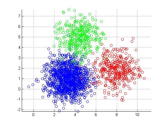
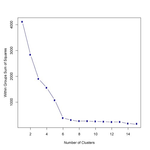
K-means: This is about clustering or dividing objects into K groups. Refer http://kamalmeet.com/machine-learning/k-means-clustering/

C-means or Fuzzy clustering: In K means we tried to make sure that an object is strictly part of a group, but this might not be possible always. C-means clustering allows some level of overlap between clusters, so an object can be 40% in one cluster and 60% in other.

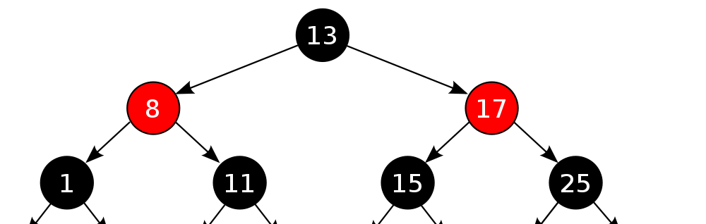
Hierarchical: As the name suggests clusters have parent child relationship and we can think of clusters as a part of hierarchical tree. Start by putting each object as individual cluster (leaf nodes) and than start combining logical cluster under one parent cluster. Repeating the process, will give us final clustering tree. For example, Orange is part of citrus fruits, which say belongs to juicy fruits, which further belongs to Fruits as top cluster.

Reinforcement Learning: In the above two learnings, we have supplied the machine information about how to come up with a solution. Reinforcement learning is different as we expect machine to learn from its experience. A reward and penalty system is in place to let machine know if the decision made was correct or incorrect to help in future decisions.

Helpful links:

https://www.analyticsvidhya.com/blog/2017/09/common-machine-learning-algorithms/

Data Gathering, Cleanup and Analysis

It is said enough times that data is to 21st century what oil was to 20th century. But as the crude oil needs to be refined, similarly data needs to be refined before it can be made useful. There are various steps involved starting from raw data to reach to a useable insight.

One often starts with a form of data which can be structured, semi-structured or unstructured. A structured data, as the name suggest is following some kind of structure, and easy to make sense of. This data might be in databases in form of tables or structured data files like excel sheets. A semi structured data also follows some structure but it is not as clean, for example a JSON or XML formatted data. All remaining data is unstructured, i.e. log files, video/ audio streams, text files etc.

When we get the data, first step is to filter out useful data. Next step is to clean up data for example removing null values by meaningful data (use mean, median or mode), cleaning up the text data, finding keywords and tags etc. Once we have all the relevant data cleaned up (tidy data along with meta data), we need to find a good sample data set for our study.

A good example of sampling is exit polls we see generally during election times. When predicting election results, a news agency cannot check with all the voters, so they have to get opinion from a sample set. It is important to choose sample data set correctly to get accurate results, for example if we have 30 percent high income groups voter, 40% middle income and 30% low income group in a constituency, whereas the news agency sampled 70% of high income group voters, they will definitely get incorrect results.

Another important aspect is data visualisation. You need to find correct form of data visualisation to make sure data reaches out and makes sense to all stake holders. Histogram, Scatter plots, Box plots, Strip charts etc are used for visualising the data.

We do have a lot of tools to help us in whole data gathering, cleanup , analysis and visualisation process. For example we can use Kafka to get the data to system.
Hadoop Map reduce / Spark handle huge amount of data and apply relevant cleaning and organising algorithms. Tools like Pig are used to clean the data and Hive to store the data. Finally
Mahut/ R/ Python reads the data and find the results to be used by stakeholders.

Conditional Probability and Bayes Theorem

Understanding probability of occurring of an event is an important part to understand in Machine learning and Data Science.

Taking a simple example, say we need to figure out probability of two dice getting rolled and sum is greater or equal to 10, i.e. sum can be 10, 11, 12. This can occur in following manner

{{4,6},{5,5},{5,6},{6,4},{6,5},{6,6}} =6

so we have 6 outcomes which can fulfill this condition.
Total outcomes

{{1,1},{1,2},…,{5,5},{5,6}} = 36

So probability of sum to be more than or equal to 10 is

desirable outcomes/ total outcomes = 6/36 = 1/6

After the simple probability, comes conditional probability. There might be some preconditions for an event to occur, which increases probability of the event to occur. For example, probability of “it will rain” gets increased if we already have an event “it will be cloudy”.

Going back to previous example, lets say we add a condition “figure out probability of two dice getting rolled and sum is greater or equal to 10 – when the first dice already has 5”

P(A)= P(A and B)/P(B)
A = Event we need to check probability for, in this case, probability of sum greater than 10 when first dice has 5
B = Event that First dice has five
A and B = probability of both events occurring together.

We already know total outcomes for two dice being rolled is 36.
Probability for Event B, i.e. first dice has 5, we have {{5,1},{5,2},{5,3},{5,4},{5,5},{5,6}}
i.e. 6/36 or 1/6
Probability for A and B, i.e. first dice has 5 and sum is greater or equal to 10 {{5,5},{5,6}}
i.e. 2/36 or 1/18

putting these values in formula

P(A)= P(A and B)/P(B)
P(A)= (1/18)/(1/6) or (6/18) or (1/3)

Finally coming to Bayes Theorem, this gives relation between conditional probability and its reverse.

P(A/B) = (P(B/A)*(PA))/P(B)
or
P(A/B)*P(B) = P(B/A)*(PA)

A good example is here

But I will stick to simpler one

You have 2 bags, say X and Y. X has 6 Green and 6 Red balls. Y has 4 Red and 8 Green Balls. one of the bags is randomly chosen and a ball is picked randomly. If the ball is Red, what is probability that it was taken from bag X.

We need to find P(Bag X/ Ball is Red)
As per Bayes we have
P(Bag X/ Ball is Red) = (P(Ball is Red/Bag X)*P(Bag X))/ P(Ball is Red)

As bag is chosen randomly, we know
P(Bag X) and P(Bag y) both is 1/2
P(Ball is Red/Bag X) = Bag X has 12 balls of which 6 are Red, so 6/12 = 1/2
P(Ball is Red) = Red ball is chosen from X bag OR Red ball is chosen from Y bag
=P(Ball is Red/Bag X)*P(Bag X) + P(Ball is Red/Bag Y)*P(Bag Y)
= 6/12*1/2 + 4/12*1/2
= 10/24 = 5/12

P(Bag X/ Ball is Red) = (P(Ball is Red/Bag X)*P(Bag X))/ P(Ball is Red)
= (1/2*1/2)/5/12 = (1/4)/(5/12) = 3/5

A few basic statistics for Machine Learning

Machine learning itself is big area, but to get started one needs to be familiar with a few basic concepts of Statistics and Probability.

Here are a few basic concepts given a set of numbers say 12, 5, 7, 17, 22, 5, 10, 2, 5, 17, 2, 11

Mean- Given a set of N numbers, mean is average of these numbers. 115/12 = 9.58

Median- Sort the list, for even items, median is sum of the middle 2 numbers divided by 2. For odd items median is the middle number.
2, 2, 5, 5, 5, 7, 10, 11, 12, 17, 17, 22
7+10= 17/2=8.5

Mode- Number that appears most often in the list. In this case it is 5.

Range- Max number minus minimum number in the list: 22-2= 20

Variance- It is the measure of how the set of number is varying from the mean. This is calculated by finding difference of each number from mean and than squaring.

Taking a simple example in this case, say we have 3 numbers, 1, 2, 3 mean in this case would be 6/3 =2. So variance would be
(1-2)^2+(2-2)^2+(3-2)^2 / 3= 2 /3 = 0.67

Standard Deviation- The variance is figured by squaring the difference of mean and numbers in list. Standard deviation takes the square root of variance to reset the unit of original list. So in case variance was 0.67, standard deviation would be sqtr(0.67) or 0.81.

K-means clustering

Clustering, as the name suggest is simply grouping some random elements. Say, you are given points on a 2-D graph, you need to figure out some kind of relationship or pattern among them. For example you might have crime position in a city or Age vs Mobile Price graph for purchasing habit of an online website.

In Machine Learning, clustering is an important class of algorithms as it helps figure out a pattern in random set of data and helps take decision based on the outcome. For example, an online store needs to send a targeted marketing campaign for new Mobile phone launched. Clustering algorithm can help figure out buying patterns and single out customers who are most likely to buy the mobile phone launched.

There are many clustering algorithms, K-means being one of the simplest and highly used.

1. Place K points randomly on the graph. These will serve as initial center points or centroids of the K clusters.
2. Now assign each item (point) existing in the graph to one K clusters, based on its closeness (shortest distance from centroid) to the centroid of cluster
3. When all items are assigned a cluster, recalculate centroid of the cluster (point from where distance to all the items in cluster is minimum on an average).
4. Repeat step 2 and 3, until there is no scope of improvement (no movement in seen in centroids).

The above algorithm will divide all the items into K clusters. Another challenge will be to come up with optimum value of K. i.e. How many clusters can correctly or adequately represent the data. Well there are many ways to figure that, one of effective way is the elbow method. You start plotting number of clusters on X axis and Sum of squared errors on Y axis. Sum of squared errors is, you take each point in a cluster, find the distance from centroid and square it (to eliminate negative distances), this is the error for this particular point as ideally you want each point near to centroid of cluster to make it perfect. Then sum up all these errors and plot on graph. The resulting graph starts looking like an arm. We find out the elbow, that is, where we see the numbers getting flatter on X axis. This means any additional cluster is not adding too much value to the information we already have.