Tag Archives: Data Structure

HashMap- Collision handling using chaining and open addressing

A HashMap is a datastructure which links a key to the value. For example key can be employee id and value might be employee details. The definition actually is true for any map, a hash map adds the functionality of hashing to a simple key-value map. A hash function maps a key to a particular bucket (we can think of it as array position) to add value. For example, if employee id is unique, a good hash function would simply return employee id itself as key. But in case, we are trying to use employee name as key, we might need a better hashing function to generate a bucket id based on employee name.

As we can see from above example, if we do not choose a good hash function, we might not be able to get unique bucket ids for every key. So multiple keys might actually return same bucket id. This causes a collision.

There are 2 important ways to handle collisions

Separate Chaining: In this technique, we create a list inside each bucket to store the objects in case one bucket needs to handle multiple objects. For example, say keys Dave and David returns same hash say bucket number 4 (or array index 4), we would create a linked list in bucket four and store both elements in the list. The advantage is that we can infinitely grow this list (provided no space concerns) and handle any level of collisions.

Open Addressing:
In this technique, if in case say two keys generate same hash, the first one would be stored at the hash position, and the other one(s) would be stored at next best position. There are again multiple ways to find the next best position. Here are 2 simple ones

Linear Probing: Simply look for next empty space in array. For previous example, say David has a hash value 4, and we found that position 4 is already filled, we will simply look for next empty position, say 5 is empty, we will save David’s object in 5 or if 5 is also booked we will move on to 6 and so on.

Double Hashing: Going to previous example, if we found bucket 4 is full, instead of simply looking for next empty position, we will invoke a new hash function and add the returned number to initial bucket number. Say input David returned 16 from second hash function, we will try to insert the object at 4+16 i.e. 20th position. If 20th position is also filled, we will move to 20+16 i.e. 36 and so on.

Worst case Analysis

The performance of a hashmap usually depends on the hashing function. For example, say we have <=1000 objects and we create a map with 1000 entries. The perfect hashing function would map each entry to a unique entry in the map. In such a case we will have addition, deletion and search at worst case as O(1). Similarly, if we choose a worse hash function, which lets say maps each key to a single bucket (say a dumb hash function return 10, no matter what the input is), we will end up with a worst case search of O(n). Because of the above reason, we cannot guarantee a worst case performance for a hashmap, and hence a Binary Search Tree or a Red Black tree would sometimes be preferred in performance critical operations, as we can guarantee a max search time. Separate Chaining vs Open Addressing An obvious question is that which collision handling technique should be used. Both has its advantages. As a thumb rule, if space is a constraint and we do have an upper bound on number of elements, we can use open addressing. The advantage with Separate chaining is that it can grow indefinitely (if space is available).

Minimum Priority Queue- Java Implementation

http://kamalmeet.com/data-structure/priority-queue/
http://kamalmeet.com/algorithms/heap-data-structure/

package com.kamalmeet.www;

/**
 * This is a sample implementation of Min Priority queue. 
 * This will work for any object type which has a valid comparable interface implemented.
 * 
 * @Copyright kamalmeet.com
 * @author kamalmeet
 *
 * @param 
 */
public class MinPriorityQueue {
  
  Type minQueue[]=null;
  int elements=0;
  
  /**
   * Constructor to create a Minimum priority queue of a specific size.
   * 
   * @param size
   */
  public MinPriorityQueue(int size){
    minQueue=(Type[]) new Object[size];
  }
  
  /**
   * A new element is always added at the last leaf and then moved up till we find correct position.
   * 
   * @param t
   */
  public void add(Type t)
  {
    if(elements==0)
    {
      System.out.println("adding"+t);
      minQueue[0]=t;
      System.out.println(minQueue[0]);
      elements++;
    }
    else
    {
      System.out.println("adding 2"+t);
      minQueue[elements]=t;
      moveUp(elements);
      elements++;
      
    }
  }
  
  /**
   * Zeroth element is deleted and returned. 
   * Last element would move to root element and queue would be heapified.
   *  
   * @return
   */
  public Type delete()
  {
    Type min=minQueue[0];
    minQueue[0]=minQueue[--elements];
    moveDown(0);
    return min;
  }
  
  /**
   * In Move up or swim method, an element is compared to its parent and moved 
   * up unless correct position is found.
   * 
   * @param num
   */
  public void moveUp(int num)
  {
    System.out.println("move:"+num);
    while(((Comparable)minQueue[num]).compareTo(minQueue[parent(num)])<0)
    {
      swap(num, parent(num));
      num=parent(num);
    }
  }
  
  /**
   * In move down or sink method, an element is compared to its children and moved 
   * down unless correct position is found.
   * 
   * @param num
   */
  public void moveDown(int num)
  {
    if(leftChild(num)>elements)
      return;
    Type leftChild=minQueue[leftChild(num)];
    if(rightChild(num)>elements)
    {
      if(((Comparable)leftChild).compareTo(minQueue[num])<0)
      {
        swap(num, leftChild(num));
        return;
      }
    }
    else{  
      Type rightChild=minQueue[rightChild(num)];
      if(((Comparable)leftChild).compareTo(rightChild)<0)
      {
       if(((Comparable)leftChild).compareTo(minQueue[num])<0)
       {
         swap(num, leftChild(num));
         moveDown(leftChild(num));
       }
      }
      else
      {
        if(((Comparable)rightChild).compareTo(minQueue[num])<0)
        {
          swap(num, rightChild(num));
          moveDown(rightChild(num));
        }
      }
    }
    
  }
  
  /**
   * Method to swap 2 elements.
   * 
   * @param i
   * @param j
   */
  public void swap(int i, int j)
  {
    Type t=minQueue[i];
    minQueue[i]=minQueue[j];
    minQueue[j]=t;
  }
  
  /**
   * Find parent of an element. usually it is element/2 but we need to take 
   * care of the fact that array starts from 0.
   * 
   * @param i
   * @return
   */
  public int parent(int i)
  {
    if(i==0 || i==1 || i==2)
      return 0;
    int p=(i+1)/2;
    return p-1;
  }
  
  /**
   * Finds left child for the element.
   * 
   * @param i
   * @return
   */
  public int leftChild(int i)
  {
    //as array starts from 0, we will need to add 1 initially and subtract 1 finally
    int c=0;
    c=(i+1)*2;
    return c-1;
  }
  
  /**
   * Find right child for the element.
   * 
   * @param i
   * @return
   */
  public int rightChild(int i)
  {
    //as array starts from 0, we will need to add 1 initially and subtract 1 finally
    int c=0;
    c=((i+1)*2)+1;
    return c-1;
  }
  
  /**
   * Method to print the minimum queue (for debug).
   */
  public void print()
  {
   
    for(int i=0;i min= new MinPriorityQueue(10);
    
    min.add(11);
    min.add(88);
    min.add(99);
    min.add(43);
    min.add(2);
    min.add(36);
    min.add(222);
    min.add(123);
    min.add(7);
    
    min.print();
    System.out.println("********************");
    System.out.println("deleted:"+min.delete());
    min.print();
    
  }

}

2-3 Trees, B Trees and B+ Trees

Recently I wrote about Binary Search Tree, AVL Tree and Red- Black trees. Here I will cover basics of other important tree structures.

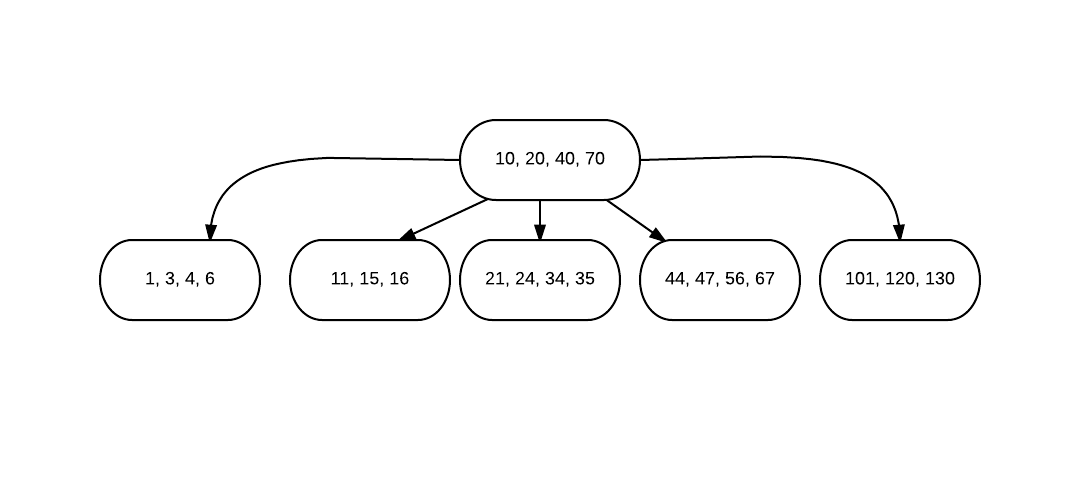
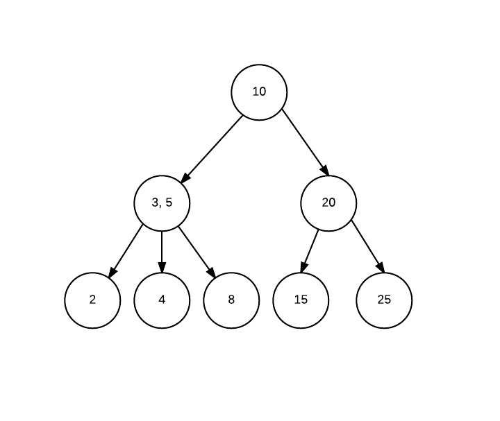
2-3 Tree: In a binary search tree, we have a restriction that each node can have 2 children. In 2-3 tree, the restriction is relaxed a bit and each node can have 2 or 3 children, and node itself can contain 1 or 2 data values. 1 data value will correspond to 2 child nodes, same as BST. In case of 2 data values, the the child nodes are divided into 3, one values smaller than left node, second child has values between first and second values, and right child has values greater than both the node values.

An Example

2-3tree

Read more here

B- Tree: B tree is modified BST or 2-3 trees to support systems which supports sequential and blocks read. Each node can store N values and have N+1 number of children.

btree

Read more here

B+ tree:
B+ tree is form of B tree with an addition that actual node values/ objects are stored at leaf nodes, and intermediary nodes only have keys used for reaching leafs.

Read more here

Red Black Tree

Sometime back I wrote about Binary Search Tree (BST) and AVL tree. AVL tree helps us maintain search at an O(log N) complexity. The price we have to pay, is to maintain balance of tree with every insertion or deletion in tree.

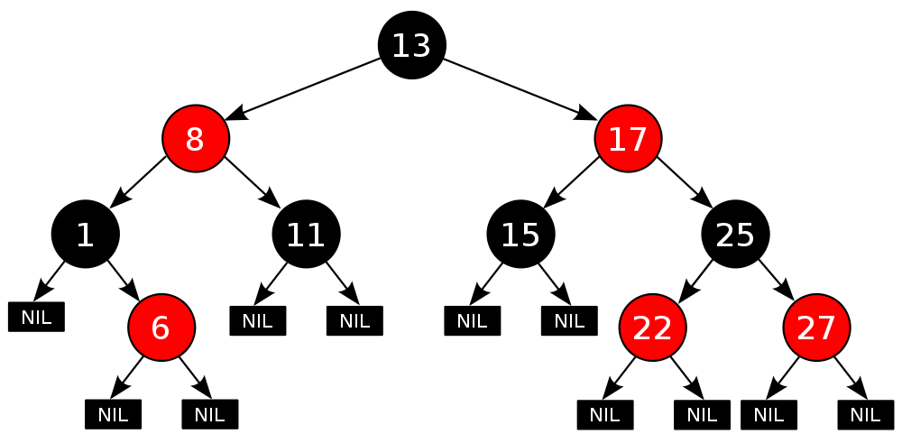
Red black tree, is another balanced BST, but not as strictly balanced as AVL. A red black tree, has following properties.

1. Each node is marked either red or black.
2. Root is always black (does not impact actually- read on)
3. Each leaf node is null and black (It is optional to show leafs, but good for initial understanding).
4. Imp- No 2 red nodes can be directly connected, or no red node can have a red parent or child.
5. Imp- A path from root to (any) leaf will always have same number of black nodes.

Property 4 & 5 makes sure we always end up in a balanced BST.

here is an example red black tree. (image from wikipedia)

red_black

Here is a good illustration of how red black tree works – http://www.cs.usfca.edu/~galles/visualization/RedBlack.html

As red black tree gives a bit flexibility over AVL in tree balancing, insert operation is faster than AVL with less number of tree rotations. The insert speed comes at a cost of a tad slower searching, though it is still O(log N), the levels can be 1 or 2 more than AVL as tree is not strictly balanced.

Further readings

http://www.geeksforgeeks.org/red-black-tree-set-1-introduction-2/


https://en.wikipedia.org/wiki/Red%E2%80%93black_tree

https://www.cs.auckland.ac.nz/software/AlgAnim/red_black.html

http://stackoverflow.com/questions/1589556/when-to-choose-rb-tree-b-tree-or-avl-tree

http://stackoverflow.com/questions/13852870/red-black-tree-over-avl-tree

Binary Search Tree and AVL Tree

In last post I mentioned about Binary Search tree. One challenge with Binary Search Tree or BST is when we try to insert a sorted list into it, we will end up a straight list structure rather than tree, i.e. we are adding all the nodes to one side. For example

bst_unbalanced

In this case, when we search for an element at extreme right, we are making O(N) comparisons.

To improve this situation, we have Balanced Binary search trees. AVL is one of such Balanced BST trees.

AVL tree has additional property over BST, that at any point of time, any 2 subtrees from a root can differ in height by order of 1. Or in other words, in a tree with height N, only last 2 level (N and N-1) of the tree can have leaf nodes without children.

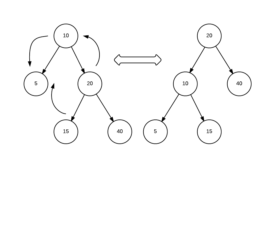
AVL Tree maintains this balance using tree rotation. We can rotate a tree (or subtree) in left or right direction.

tree_rotation

The above example shows how left rotation works (if you look other way around, swap source and destination, it is right rotation).

More on tree rotation- https://en.wikipedia.org/wiki/Tree_rotation

Additional reads
https://en.wikipedia.org/wiki/AVL_tree

http://www.geeksforgeeks.org/avl-tree-set-1-insertion/

http://stackoverflow.com/questions/14670770/binary-search-tree-over-avl-tree

A very good visual representation of AVL tree Vs Binary tree. Try creating a tree with nodes 1,2,3,4,5,6,7,8,9 and see visual difference between 2 trees. http://visualgo.net/bst.html#

Binary Search Tree

To start with, lets understand what a tree datastructure is. A tree supports one way relation between objects of similar type. A very real example would be the way file system stores directories and files. A directory can have files as well as other directories which in turn can have more directories and files.

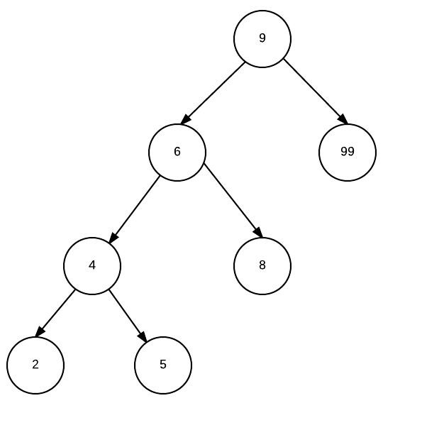
A Binary tree puts a restriction on tree that any node can have only 2 childs.

bst

A Binary search tree adds a property to binary tree that each node on left of parent node will have less key value than parent and each node on right will be higher key value. In turn, this also means at any point of time, for a node, whole left sub tree will have lower keys than the node value and right subtree will have higher values.

The above mentioned property helps in search operation. Lets say we are seaching for N

1. Go to root Node R.
2. Check if N is equal to R, return true.
3. if N>R, N=N.right (discard left tree)
4. if N

Kruskal’s Algorithm for Minimum spanning tree.

In last post I talked about Prim’s algorithm for minimum spanning tree.

Kruskal is another alorithm to solve same problem.

1. To start with, remove all edges from graph.
2. Add edges to a set S in sorted order with increasing order of weight.
3. Take an edge from set S (next minimum weight) and add to graph if (and only if) it is connecting non- cnnected nodes. Igore the edge if vertices are already connected.

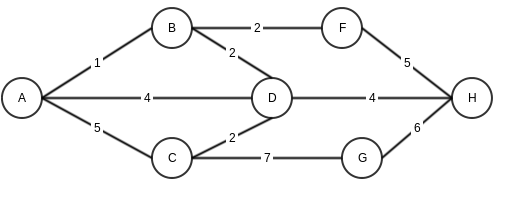
So if I try to same problem for this graph.

graph

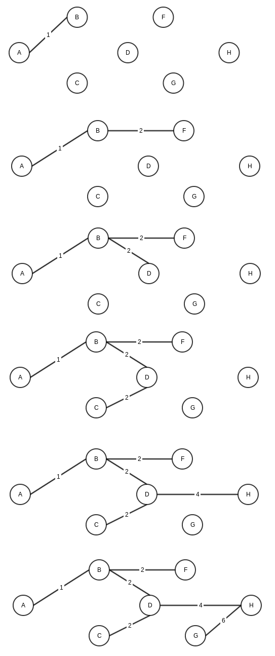
These will be the steps

kruskals

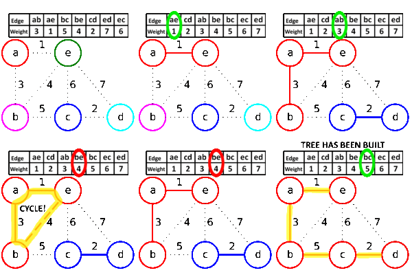
Another interesting depiction from wikipedia

kruskal2

Prim’s Algorithm for Minimum spanning tree.

If we look at wikipedia for Prim’s alogorithm, it states

“Prim’s algorithm is a greedy algorithm that finds a minimum spanning tree for a weighted undirected graph”

https://en.wikipedia.org/wiki/Prim%27s_algorithm

Let’s take this line word by word

Greedy algorithm: means this algorithm looks at the best option available at current stage and move stage by stage.

weighted graph: a graph where edges have a weight associated, for example distance as weight in case of a graph showing path between cities.

undirected graph: A graph which does not worry about direction of edges. A edge between vertices A and B would mean it can travel both ways.

Minimum spanning tree: In a graph, a minimum spanning tress is a tree, which has only edges which are required to connect all the nodes and keeping minimum weight.

Now Coming to Prim’s algo, again using wikipedia’s definition

    1. Initialize a tree with a single vertex, chosen arbitrarily from the graph.
    2. Grow the tree by one edge: of the edges that connect the tree to vertices not yet in the tree, find the minimum-weight edge, and transfer it to the tree.
    3. Repeat step 2 (until all vertices are in the tree).

Let’s say we have a graph

graph

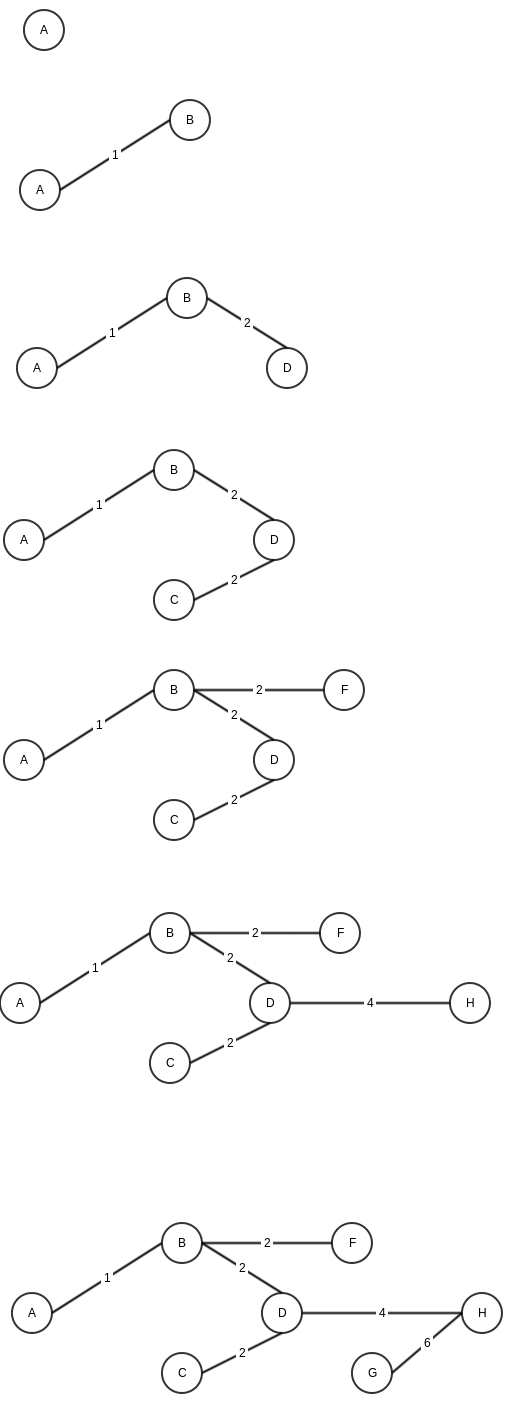
Here is step by step execution of Prim’s algorithm (note that for steps where we have multiple same minimum weight options, I am choosing randomly)

prims

Priority Queue

A queue is FIFO datastructure which means objects added first will be accessed first. Priority queue adds an element of priority with each object added to queue. And when elements are accessed they will be accessed based on this priority in increasing (min- priority queue) or decreasing (max- priority queue).

There are multiple ways we implement priority queue, basic one is to use queue, and just add priorit elelemnt. A queue has insertion and deletion operation at Order of 1 as elements are added and removed from front. But in case of priority queue, though we will add elements at front, but delete/ fetch based on priority, so we will need to traverse the whole list, hence O(N).

Start->Node1{obj, P3}->Node1{obj, P4}->Node1{obj, P1}->Node1{obj, P2}->End

Another, more efficient way to implement priority queue is using heap data structure.

Read here about – http://kamalmeet.com/algorithms/heap-data-structure/

As heap data structure automatically maintains priority (Min heap – Min priority queye/ Max heap – Max priority queue), it fits best to implement priority queue. As both insertion and deletion of objects in heap is O(log N) operation, same is true for priority queue implemented through heap.

Graph Data Structure

Graph is distant relative of Tree. Infact it is complexer than tree, as in tree, a node usually have link with nodes one level up or down and does not conatin any cycles, whereas graph does not have any such restrictions. Graph data structure is more useful in case of something like traveling salesman problem, or to represent computer network, i.e. a structure where we have nodes and relationship between them.

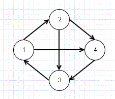
graph

In the above graph structure, we have 4 nodes or Vertices and 6 Edges (connectors). A graph is usually represented as G=(V,E).

Please note that the graph given above is directed, that is we can see link is from 1->2 and not 2->1. In undirected graph, the arrows showing direction of connection will not be there and connection can be considered both ways.

Adjacency Matrix

The above graph can be shown as

[1] [2] [3] [4]
[1]   0    1     0    1
[2] 0 0 1 1
[3] 1 0 0 0
[4] 0 0 1 0

if the same graph was undirected
[1] [2] [3] [4]
[1] 0 1 1 1
[2] 1 0 1 1
[3] 1 1 0 1
[4] 1 1 1 0

Always Aij=Aji in undirected

Adjacency List Representation

Node1->[Node2, Node4]
Node2->[Node3, Node4]
Node3->[Node1]
Node4->[Node3]

Other useful information for Graphs

Degree: Number of edges being attached to current vertex
In-Degree: Number of edges coming into the vertex in case of directed graph
Out-Degree: Number of edges going out from the vertex in case of directed graph

Weighted Graphs:

This is important in case we are trying to solve problems like traveling salesman. For example, if we look at above graph, we can see there are 2 ways to reach Vertex 3 from Vertex 1, that is, 1->4 or 1->2->4. Say these vertices represent cities, and edge weight represent distance in this case.

1->2= weight 20
2->4= 30
1->4= 60

So we can choose 1->2->4 over 1->4 as it will be shorter distance.