Category Archives: Decision Making

Decision Making Under Certainty

There can be cases where we have all the needed data is available, and we need to make decisions such that a given objective is achieved in the best possible manner while satisfying conditions imposed.

To understand the concept let’s take the problem of optimizing resource utilization and maximizing profit, where we have all the details on how much resources are being used by the products. Say in a factory, we are building 2 products, Product A and B. The Factory has 4 units. Product A generates 30000 in profit and manufacturing needs 1 hr in unit 1, 2 hr in unit 2, and 2 hr in unit 3. For product-B, it generates 50000 in profit and its manufacturing needs 2 hr in unit 1, 2 hr in unit 2, and 3 hrs in unit 4. As given constraints, we know that unit 1 can operate 4000 hrs, unit 2 can operate 6000 hrs, unit 3 can operate 5000 hrs and unit 4 can operate 4500 hrs in a month.

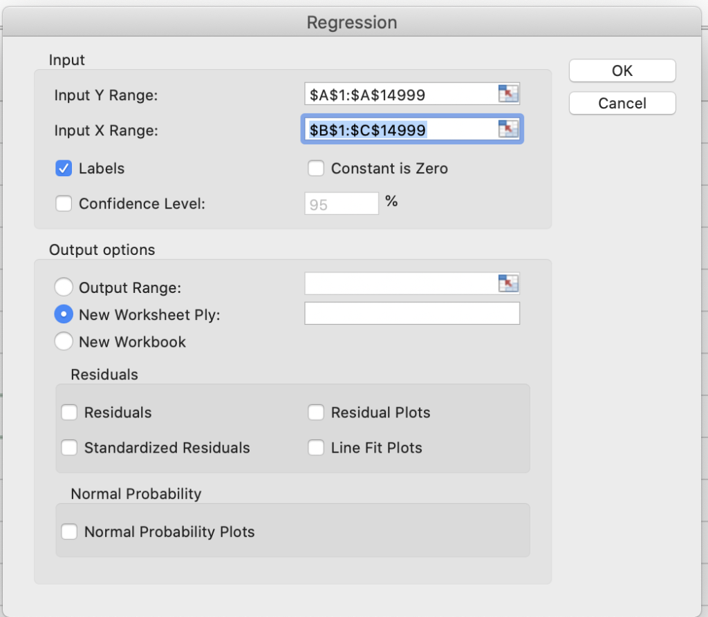
To solve this problem, we are going to use the Simplex Linear Programming method. This is available off the shelf in Microsoft Excel, so we will set up the data in an excel sheet.

Simplex LP

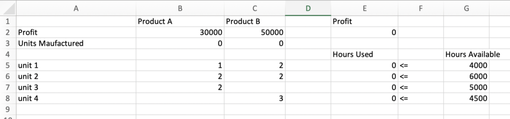
Let’s try to understand the data here before moving ahead. We have added data for Product A and B, Profit data for per unit, units manufactures is just a placeholder for now, and then we have given the number of hours spent in each unit by both the products.

Column E2 has total profit, i.e. number of units for product A * per unit profit product A + number of units for product B * per unit profit product B or =SUMPRODUCT(B2:C2, B3:C3)

Column E5 to E8 is also dynamically calculated. For example, E5 has Time spent by product A in unit 1 * units manufactured Product A + Time spent by product B in unit 1 * units manufactured Product B or B5 * B3+ C5 *C3. Similarly, E6,7 and 8 are calculated.

Once we have an excel setup, the next steps are easy. Go to Data -> Solver -> Object (choose column E2 where we calculate total profit) -> For “To”, let the default max be selected as we want to maximize profit -> For Changing variable cells choose B3 and C3 where we have units manufactured for A and B -> Add constraints by selecting Hours available cell reference i.e. from E5 to E8 is <= G5 to G8 (constraints can be added one by one or in one go when the comparison is same i.e. in this case <=) -> Choose Solving method as Simplex LP.

When you click on solve, you will get an optimal solution

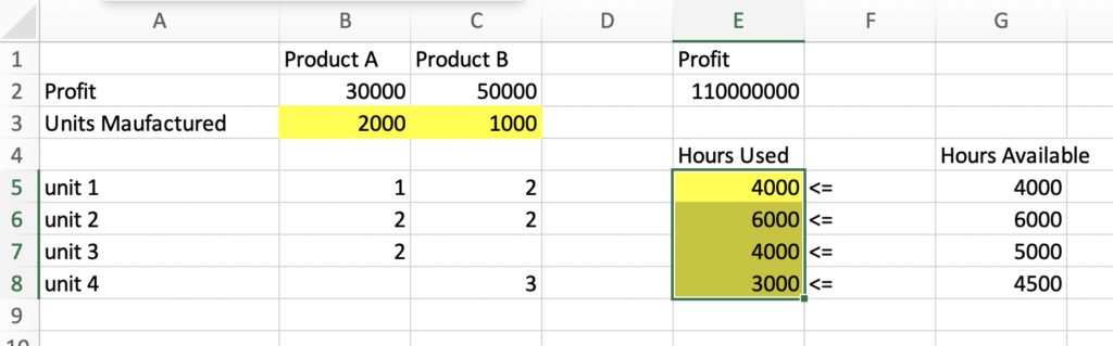
The solution says that we should produce 2000 units of product A and 1000 units of product B with a maximized profit of 110000000.

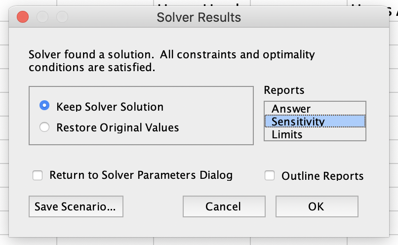
Now there can be situations like due to some operational issue we lost 100 hrs in unit 1 or there is a way we can borrow 100 hours for unit 2 from another factory, what is the impact on our profit. Or say due to change in market dynamics product A can give a profit of 40K instead of 30 K. An valuable tool to look at all the related data is sensitivity analysis. When we clicked solve button on Solver, we are given an option to generate a sensitivity analysis report.

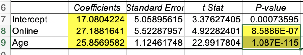
The generated report looks like

sensitivity analysis

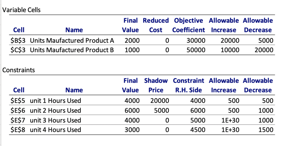
The upper 2 rows here talk about 2 products. So coming back to our question, that if instead of 30K, we get a profit of 40K from product A, shall that change my product mix. The report says that there is no impact on product mix for increase by 20 K or decreases by 5K, or in other words, product A profit can range from 25K to 50K and current product mix remains valid. Similarly for Product B, the profit range is 30K to 60K. Any change beyond this will need us to recalculate the analysis.

Coming to Constraint data, shadow price indicates that each hour in the current unit has this much impact. For example, if we can increase unit one capacity by one hour, from 4000 to 4001, we can increase our profit by 20K, so getting extra 100 hours will result in 2000K, and reduction by 100 hours will have the same negative impact on profit. The range of increase and decrease of 500 each says that the calculation is valid till this range, so if we say unit one can get more than 500 hours, we will need to recalculate the values as the current calculation will no more hold good.

Hypothesis Testing for Decision Making

In the last post. when I talked about Sampling and Estimation, we discussed P-Value in regression analysis and how this should be less than our error threshold α (alpha). We will understand what is this α value and how we get this while understanding the hypothesis testing.

Hypothesis testing is all about coming up with a hypothesis and figure out if should reject or not. The two components we have here are

  • Null Hypothesis or H0
  • Alternate Hypothesis or H1

Conditiions

  1. Together the two hypotheses should cover all possible outcomes
  2. The two hypotheses should be mutually exclusive.

α is the tolerance level or level of accepting the error. so we can say

P-Value or Probability of current outcome <= α [Reject H0]
P-Value or Probability of current outcome > α [Do not Reject H0]

Reject H0Do not Reject H0
H0 is TrueType 1 ErrorOK
H0 is FalseOKType 2 Error
Hypothesis testing

α is Probability of Type 1 Error.

Let’s take an example, the judiciary system says “innocent till proven guilty”. So consider this as the null hypothesis

H0 Person is innocent (we need to reject this to prove the person is guilty)
H1 Person is guilty

Type 1 Error: Person is innocent but is treated guilty (we target to minimize this)
Type 2 Error: Person is guilty but is treated innocent

Sampling and Estimation

An important tool for decision-making is sampling and estimation. For any promotional campaign, new product launch strategy, marketing ad campaign, etc. companies need to understand their customer behavior. Sampling and estimation is a strong tool to analyze the customer’s data, for example, say a supermarket company wants to understand how profitable is an online customer vs an offline customer. Rather than going through data for all the customers a random sample is taken and analyzed.

Sample Data snapshot

Data Analysis: Let’s say we are able to calculate following data

Sample Size: 14998
Profit for Sample: 1665295
Average: 111.03
Standard Deviation: 275.30

Similarly we can find data for Online vs Offline Customers

Online Customers

Sample Size: 3830
Profit for Sample: 448509
Average: 117.13
Standard Deviation: 283.91

Offline Customers

Sample Size: 11168
Profit for Sample: 1216786
Average: 108.94
Standard Deviation: 272.27

Point Estimates vs Interval Estimates

The above estimate that we have done is a form of a point estimate as we are trying to find an average point and use it as an estimator for the population. For example, we have an average profit estimate for online customers is 117.13. But it is highly unlikely that an online customer’s profit is actually 117.13. So we try to find a range or interval in which the profit is likely to fall. An important aspect of such an analysis is how confident are we with our range. Normally such an analysis is done for confidence levels at 90%, 95% (mostly used), and 99%.

90% Confident Interval (CI) = (sample mean – 1.645* SD/√sample size, sample
mean + 1.645* SD/√sample size)

95% Confident Interval = (sample mean – 1.96* SD/√sample size, sample
mean + 1.96* SD/√sample size)

99% Confident Interval = (sample mean – 2.576* SD/√sample size, sample
mean + 2.576* SD/√sample size)

Let’s solve for online customers CI level 95%

117.13 – 1.96*275.30/√3830 , 117.13 + 1.96*275.30/√3830

108.41, 125.84

Simple Regression Analysis

An important tool for analysis is simple regression, where we try to predict a dependent variable based on the value of the independent variable. The equation would look like

y = mx + c

You might recognize this equation as an equation for a line in the 2D plane. So basically we try to plot all the points on the 2D plane and try to figure out a pattern.

y is the dependent variable
x is the independent variable
m is slope
c is intercept

To solve this, Microsoft Excel provide us off the shelf tool for Regression.

Go to Data-> Data Analysis -> Select Regression -> For Y range choose Profit Column -> For X Range choose Online/ Offline Column -> Select Labels checkbox as we have selected header row as well -> Let confidence level default and press OK

Output of Simple regression is

Important values to note here is coefficients, which we can substitute in our equation

y = mx + c
c= 108.94
m = 8.19

x can be online or offline in our case we have values 0 or 1

so for online (x=1) customers, equation resolves to

Profit for online customers = 8.19 * 1 + 108.94 = 117.13

Profit for offline customers = 8.19 * 0 + 108.94 = 108.94

This is ins sync with our earlier calculations.

An important value to note here is P-value. A higher P-value indicates the probability of error in the current analysis. We define a threshold α (alpha), and we keep the p-value below this threshold. I will discuss hypothesis threshold α later, but for now, we can say that a value of 11 is a very high probability of error. So this indicates can we actually associate profit with online or offline parameters. Or are there other parameters that are playing a role?

To understand this, let’s introduce another factor “age” in calculations and solve using multiple regression.

Multiple Regression Analysis

Let’s say we introduce the age data to our excel, and the data is not absolute age but say range id (when you fill a form it gives you ranges 10-18, 19-24, and so on).

Sample Data

We will repeat the steps to calculate regression, just that this time we will select both online and age column for value of x

Multiple Regression

Once calculates, we will see values like

Multiple Regression

As we can see the P-value this time is very low, we can trust our analysis. We have multiple independent variables, so our equation will be like

y = m1x1 + m2x2 + c

or Profit = 27.181 * online + 25.85 * age + 17.080

We can substitute values and find the Profit, for example, we want to find profit for young people (age group 1)

Profit Online = 27.181 * 1 + 25.85 * 1 + 17.080 =70.03

Profit Offline = 27.181 * 0 + 25.85 * 1 + 17.080 =42.85

We can calculate profit for other age groups as well. We can conclude that both age and mode (online/offline) are playing a role in profit.

Decision Trees for Decision Making

We have talked about the basics of decision making and sensitivity analysis. Next, we will look into the usefulness of decision trees in process of decision making.

We will go back to our previous example where we are analyzing between 2 product prototypes, and have probabilities and outcomes available. We will represent the data in form of a decision tree and solve the problem.

Before getting into the problem, we need to understand the basic constituents of a decision tree.

Circular nodes: shows various outcomes, for making the decision we calculate the best option based on values of available outcomes and probability

Square Nodes: These are decision nodes, which shows various options available and we need to choose the best

While drawing the decision tree, we go from left to right, but when solving the tree, we go from right to left, calculating one layer at a time. Let’s go back to our example and see the decision tree in action.

Decision Tree

We start by creating a tree, mentioning all the options available and their outcomes in case the option is chosen. Then we start solving from right to left and update values for circular – outcome nodes (values in red). We move one step backward and at the decision node, the best option is chosen.

Sensitivity Analysis in Decision Making

A few days back I wrote about the basics of decision making. Next, we will look into Sensitivity analysis.

Sensitivity Analysis examines how our decision might change with different input data.

We will start with our previous example, where a company is trying to launch a product and they have the following options right now.

ALTERNATIVESUCCESS OUTCOMEFAILURE OUTCOME
Go with prototype 1200,000-180,000
Go with prototype 2100,000-20,000
Do nothing00
Decision/ Payoff Table

Let us say

P = Probability of a favourable market i.e. Success

(1-P) = Probability of unfavourable market i.e. failure

Sensitivity Analysis

EMV Prototype 1 = 200000P – 180000(1-P)
= 380000P – 180000

EMV Prototype 2 = 100000P – 20000(1-P)
= 120000P – 20000

EMV Do nothing = 0P – 0(1-P) = 0

sensitivity analysis

Point 1

EMV Do nothing = EMV Prototype 2
0 = 120000P – 20000
P = 20000/120000
P = 0.167

Point 2

EMV Prototype 2 = EMV Prototype 1
120000P – 20000 = 380000P – 180000
P = 160000/260000
P = 0.615

So based on sensitivity analysis we can conclude based on probability of success or favorable market P, that

Do nothing if P < 0.167
Go for prototype 1 if P>=0.167 and P<0.615
Go for Prototype 2 if P>= 0.615

Decision Making – Fundamentals

What is a good decision?

A good decision is based on logic, consider all available data and possible alternatives, and is obtained through rational analysis of data and alternatives.

Does a good decision always result in favorable outcome?

No. Remember, at times good decisions can fail and bad decisions can be a success.

Steps in Decision making

  1. Clearly define the problem: Do we understand the problem or stuck at symptoms?
  2. List the possible alternatives: What options are available? Doing nothing is also an alternative.
  3. Identify the possible outcomes (or states of nature): What outcomes are possible for the alternatives figured out in step 2? Identify each outcome, positive or negative.
  4. List the payoff or profit of each combination of alternatives and outcomes: Create a matrix for each alternative + outcome combination, and figure out payoff.
  5. Select one of the decision theory models
  6. Apply the model and make your decision

Let’s say a book company is planning to launch an ebook reader (like Kindle). they have 2 prototypes currently in RnD.

Problem statement: Come up with a ebook reader which can boost sales for ebooks.

  • Alternative 1: Launch Prototype 1
  • Alternative 2: Launch Prototype 2
  • Alternative 3: Do not launch a product

Now say for each alternatives we can have various outcomes

  • Huge Success (Sales above 100K in a quarter)
  • Moderate Success
  • Failure

After this we will analyze each combination of payoffs, for example

Alternative 1 (Prototype 1) + Outcome 1 (Huge Success) = Payoff (Profit 200K, selling 100K readers)

Similarly a matrix is created for each combination possible,.

Before making a decision, one needs to take into account the Risk-taking ability of the person or organization. We can divide risk nature into

  • Risk Averese
  • Risk Nuetral
  • Risk Lovers

Also, the risk appetite will change based on the risk involved, for example, for someone earning 100K, a risk of 1K is low, but when the same risk becomes high when it involves 200K.

In addition, one also needs to take Decision making environment into consideration

Decision making Environments

  1. Decision making under certainty: Decision-maker knows with certainty the consequences of every alternative
  2. Decision making under uncertainty: decision-maker does not know probabilities of various outcomes
  3. Decision-making under risk: Decision-maker knows the probabilities of various outcomes.

In short, when a company needs to make a decision, it will start from a decision under an uncertainty position, and try to move to the decision under risk by associating some probabilities to the outcomes based on past experience or market research. When the probability is straight 1 or 0, it is a decision under certainty, which is almost never possible.

Let’s go back to our previous example, and make it simple with just 2 outcomes, and based on past experience company can predict a 50-50 chance of success or failure.

AlternativeSuccess OutcomeFailure Outcome
Go with prototype 1200,000-180,000
Go with prototype 2100,000-20,000
Do nothing00
Decision/ Payoff Table

So considering this a Decision under risk scenario, we use a popular method called Expected Monetary Value, to evaluate the alternatives.

EMV or Expected Monitory Value (alternative i) = (payoff of first outcome) * (probability of first outcome) + (payoff of second outcome) * (probability of second outcome) + ….. +(payoff of Nth outcome) * (probability of Nth outcome)

Going back to our use case, we can say

EMV for prototype 1: (0.5)*(200,000) + (0.5) *(-180,000) = 10,000

EMV for prototype 2: (0.5)*(100,000) + (0.5) *( -20,000)=40,000

EMV for Do nothing: (0.5)*0 + (0.5)*0= 0

So based on our analysis, we can see prototype 2 has the largest EMV and is the best option to go under current circumstances.