Sometime back I wrote about Binary Search Tree (BST) and AVL tree. AVL tree helps us maintain search at an O(log N) complexity. The price we have to pay, is to maintain balance of tree with every insertion or deletion in tree.

Red black tree, is another balanced BST, but not as strictly balanced as AVL. A red black tree, has following properties.

1. Each node is marked either red or black.
2. Root is always black (does not impact actually- read on)
3. Each leaf node is null and black (It is optional to show leafs, but good for initial understanding).
4. Imp- No 2 red nodes can be directly connected, or no red node can have a red parent or child.
5. Imp- A path from root to (any) leaf will always have same number of black nodes.

Property 4 & 5 makes sure we always end up in a balanced BST.

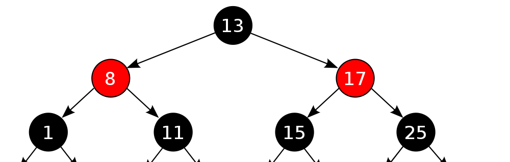
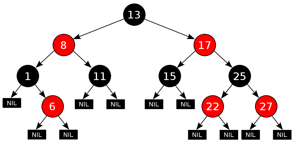
here is an example red black tree. (image from wikipedia)

Here is a good illustration of how red black tree works – http://www.cs.usfca.edu/~galles/visualization/RedBlack.html

As red black tree gives a bit flexibility over AVL in tree balancing, insert operation is faster than AVL with less number of tree rotations. The insert speed comes at a cost of a tad slower searching, though it is still O(log N), the levels can be 1 or 2 more than AVL as tree is not strictly balanced.

Further readings

http://www.geeksforgeeks.org/red-black-tree-set-1-introduction-2/

https://en.wikipedia.org/wiki/Red%E2%80%93black_tree

https://www.cs.auckland.ac.nz/software/AlgAnim/red_black.html

http://stackoverflow.com/questions/1589556/when-to-choose-rb-tree-b-tree-or-avl-tree

http://stackoverflow.com/questions/13852870/red-black-tree-over-avl-tree

In last post I mentioned about Binary Search tree. One challenge with Binary Search Tree or BST is when we try to insert a sorted list into it, we will end up a straight list structure rather than tree, i.e. we are adding all the nodes to one side. For example

In this case, when we search for an element at extreme right, we are making O(N) comparisons.

To improve this situation, we have Balanced Binary search trees. AVL is one of such Balanced BST trees.

AVL tree has additional property over BST, that at any point of time, any 2 subtrees from a root can differ in height by order of 1. Or in other words, in a tree with height N, only last 2 level (N and N-1) of the tree can have leaf nodes without children.

AVL Tree maintains this balance using tree rotation. We can rotate a tree (or subtree) in left or right direction.

The above example shows how left rotation works (if you look other way around, swap source and destination, it is right rotation).

More on tree rotation- https://en.wikipedia.org/wiki/Tree_rotation

Additional reads
https://en.wikipedia.org/wiki/AVL_tree

http://www.geeksforgeeks.org/avl-tree-set-1-insertion/

http://stackoverflow.com/questions/14670770/binary-search-tree-over-avl-tree

A very good visual representation of AVL tree Vs Binary tree. Try creating a tree with nodes 1,2,3,4,5,6,7,8,9 and see visual difference between 2 trees. http://visualgo.net/bst.html#

To start with, lets understand what a tree datastructure is. A tree supports one way relation between objects of similar type. A very real example would be the way file system stores directories and files. A directory can have files as well as other directories which in turn can have more directories and files.

A Binary tree puts a restriction on tree that any node can have only 2 childs.

A Binary search tree adds a property to binary tree that each node on left of parent node will have less key value than parent and each node on right will be higher key value. In turn, this also means at any point of time, for a node, whole left sub tree will have lower keys than the node value and right subtree will have higher values.

The above mentioned property helps in search operation. Lets say we are seaching for N

1. Go to root Node R.
2. Check if N is equal to R, return true.
3. if N>R, N=N.right (discard left tree)
4. if N

A queue is FIFO datastructure which means objects added first will be accessed first. Priority queue adds an element of priority with each object added to queue. And when elements are accessed they will be accessed based on this priority in increasing (min- priority queue) or decreasing (max- priority queue).

There are multiple ways we implement priority queue, basic one is to use queue, and just add priorit elelemnt. A queue has insertion and deletion operation at Order of 1 as elements are added and removed from front. But in case of priority queue, though we will add elements at front, but delete/ fetch based on priority, so we will need to traverse the whole list, hence O(N).

Start->Node1{obj, P3}->Node1{obj, P4}->Node1{obj, P1}->Node1{obj, P2}->End

Another, more efficient way to implement priority queue is using heap data structure.

Read here about – http://kamalmeet.com/algorithms/heap-data-structure/

As heap data structure automatically maintains priority (Min heap – Min priority queye/ Max heap – Max priority queue), it fits best to implement priority queue. As both insertion and deletion of objects in heap is O(log N) operation, same is true for priority queue implemented through heap.